You can not select more than 25 topics
Topics must start with a letter or number, can include dashes ('-') and can be up to 35 characters long.
|
|
9 years ago | |
|---|---|---|
| R | 9 years ago | |
| README_figs | 9 years ago | |
| man | 9 years ago | |
| tests | 9 years ago | |
| .Rbuildignore | 9 years ago | |
| .gitignore | 9 years ago | |
| .travis.yml | 9 years ago | |
| CONDUCT.md | 9 years ago | |
| DESCRIPTION | 9 years ago | |
| LICENSE | 9 years ago | |
| NAMESPACE | 9 years ago | |
| README.Rmd | 9 years ago | |
| README.md | 9 years ago | |
| ggalt.Rproj | 9 years ago | |
README.md
ggalt : Alternate/Extra 'Geoms', 'Stats' and 'Coords' for 'ggplot2'
A package containing additional/alternate 'geoms', 'coords' and 'stats' for use with the revamped (late 2015) version of ggplot2.
The first three forays into this brave, new ggplot2 world are splines! and being able to use the (much better) KernSmooth::bkde and KernSmooth::bkde2D for density plots and an initial port of the (still needing work) coord_proj.
NOTE
Until the new ggplot2 version is on CRAN, you'll need to install it from github (see below).
The following functions are implemented:
coord_proj: Likecoord_maponly better:-)geom_xspline: Connect control points/observations with an X-splinestat_xspline: Connect control points/observations with an X-splinegeom_bkde: Display a smooth density estimate (usesKernSmooth::bkde)stat_bkde: Display a smooth density estimate (usesKernSmooth::bkde)geom_bkde2d: Contours from a 2d density estimate. (usesKernSmooth::bkde2D)stat_bkde2d: Contours from a 2d density estimate. (usesKernSmooth::bkde2D)stat_ash: Compute and display a univariate averaged shifted histogram (polynomial kernel) (usesash::ash1/ash::bin1)
News
- Version 0.0.4.9000 released -
stat_ash - Version 0.0.3.9000 released -
coord_proj! (requires my github copy of ggplot2 for now) - Version 0.0.2.9005 released - cleanup before blog post
- Version 0.0.2.9002 released - working 2D density plots
- Version 0.0.2.9000 released
Installation
# you'll want to see the vignettes, trust me
devtools::install_github("hadley/ggplot2", build_vignettes=TRUE)
devtools::install_github("hrbrmstr/ggalt")
Usage
library(ggplot2)
library(gridExtra)
library(ggalt)

# current verison
packageVersion("ggalt")
#> [1] '0.0.3.9000'

set.seed(1492)
dat <- data.frame(x=c(1:10, 1:10, 1:10),
                  y=c(sample(15:30, 10), 2*sample(15:30, 10), 3*sample(15:30, 10)),
                  group=factor(c(rep(1, 10), rep(2, 10), rep(3, 10)))
)

ggplot(dat, aes(x, y, group=group, color=group)) +
  geom_point() +
  geom_line()

ggplot(dat, aes(x, y, group=group, color=factor(group))) +
  geom_point() +
  geom_line() +
  geom_smooth(se=FALSE, linetype="dashed", size=0.5)

ggplot(dat, aes(x, y, group=group, color=factor(group))) +
geom_point(color="black") +
geom_smooth(se=FALSE, linetype="dashed", size=0.5) +
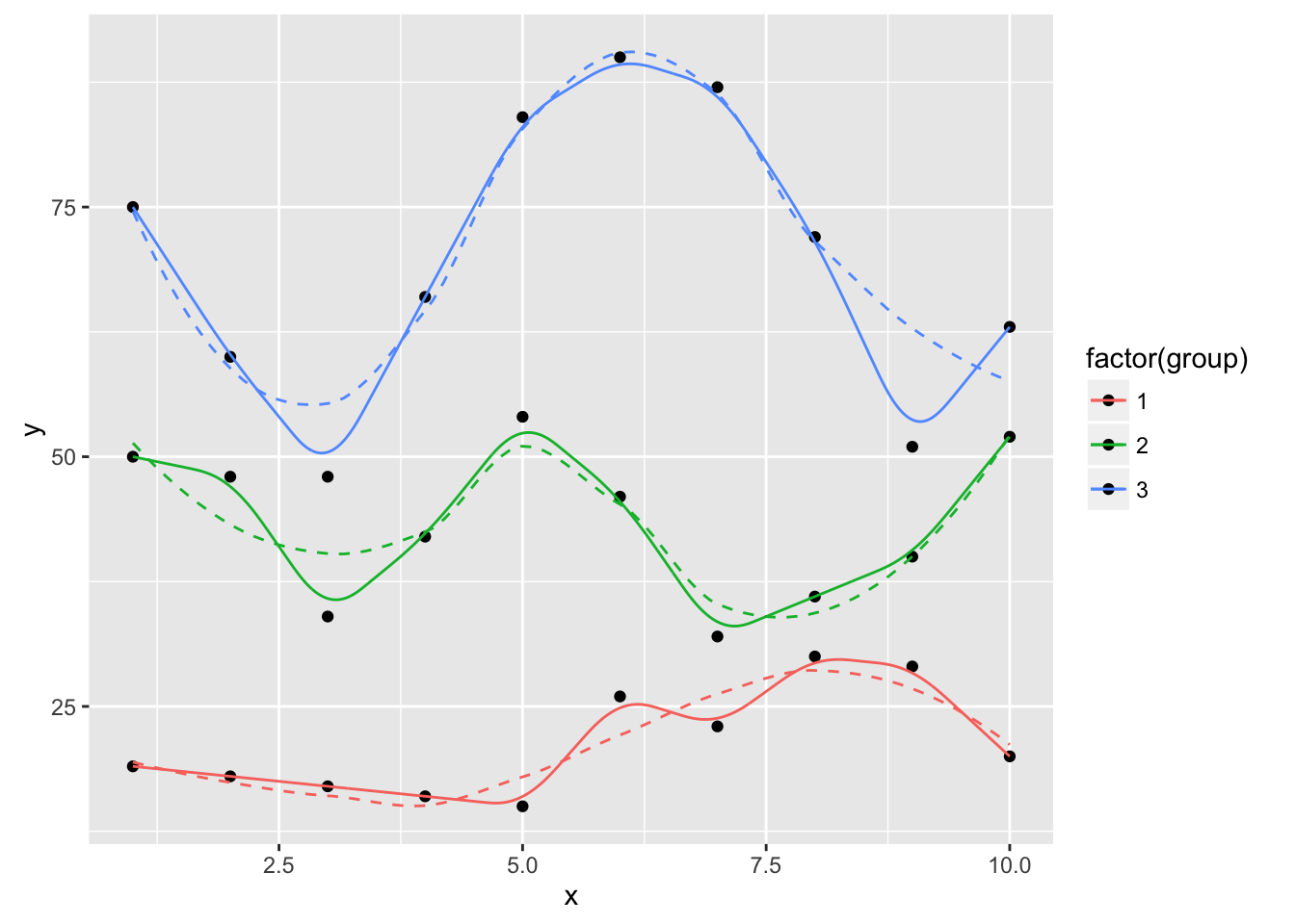
geom_xspline(size=0.5)

ggplot(dat, aes(x, y, group=group, color=factor(group))) +
  geom_point(color="black") +
  geom_smooth(se=FALSE, linetype="dashed", size=0.5) +
  geom_xspline(spline_shape=-0.4, size=0.5)

ggplot(dat, aes(x, y, group=group, color=factor(group))) +
  geom_point(color="black") +
  geom_smooth(se=FALSE, linetype="dashed", size=0.5) +
  geom_xspline(spline_shape=0.4, size=0.5)
ggplot(dat, aes(x, y, group=group, color=factor(group))) +
  geom_point(color="black") +
  geom_smooth(se=FALSE, linetype="dashed", size=0.5) +
  geom_xspline(spline_shape=1, size=0.5)

ggplot(dat, aes(x, y, group=group, color=factor(group))) +
  geom_point(color="black") +
  geom_smooth(se=FALSE, linetype="dashed", size=0.5) +
  geom_xspline(spline_shape=0, size=0.5)

ggplot(dat, aes(x, y, group=group, color=factor(group))) +
  geom_point(color="black") +
  geom_smooth(se=FALSE, linetype="dashed", size=0.5) +
  geom_xspline(spline_shape=-1, size=0.5)

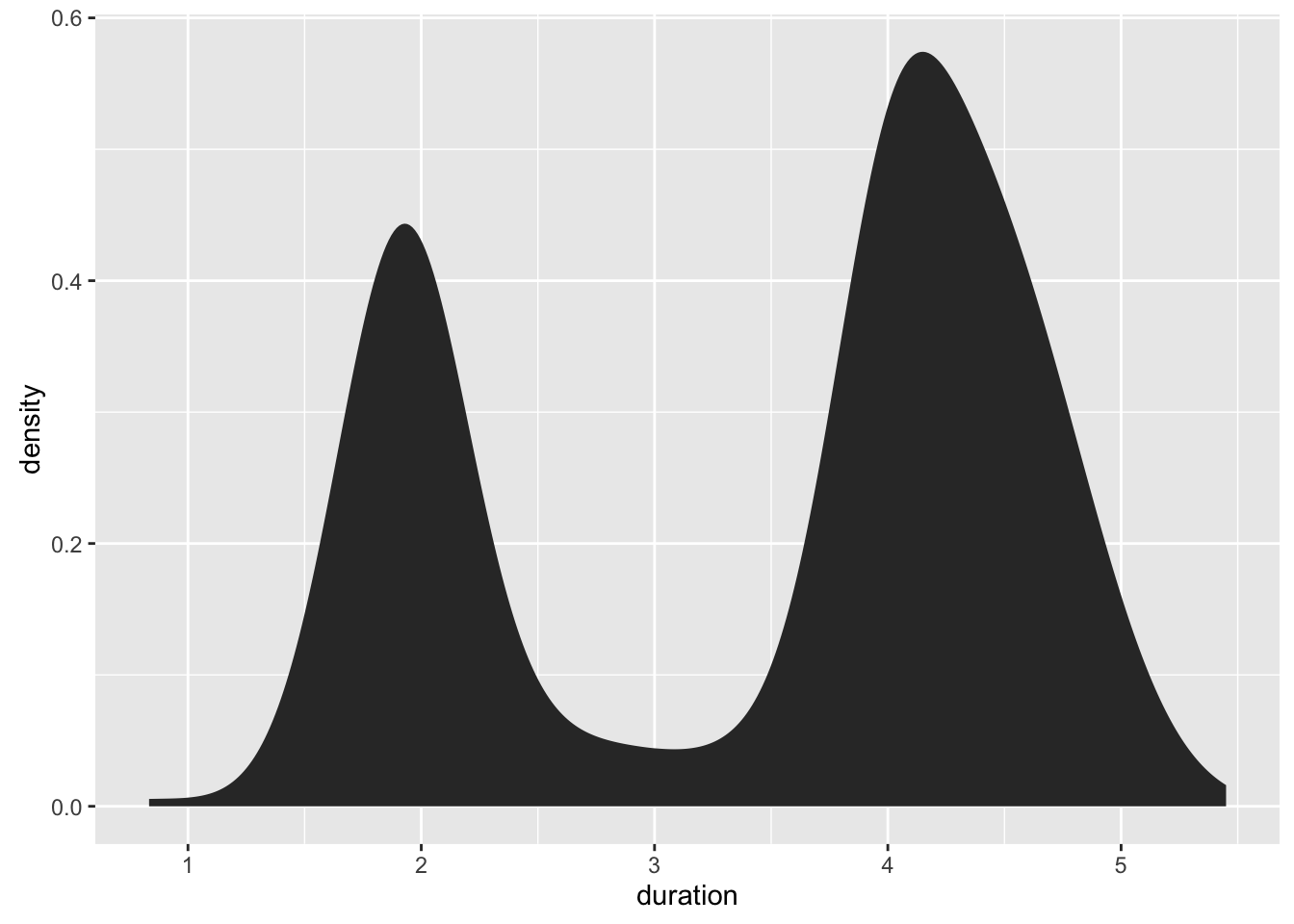
# Better density plots

data(geyser, package="MASS")

ggplot(geyser, aes(x=duration)) +
  stat_bkde(alpha=1/2)
#> Bandwidth not specified. Using '0.14', via KernSmooth::dpik.

ggplot(geyser, aes(x=duration)) +
  geom_bkde(alpha=1/2)
#> Bandwidth not specified. Using '0.14', via KernSmooth::dpik.

ggplot(geyser, aes(x=duration)) +
  stat_bkde(bandwidth=0.25)

ggplot(geyser, aes(x=duration)) +
  geom_bkde(bandwidth=0.25)
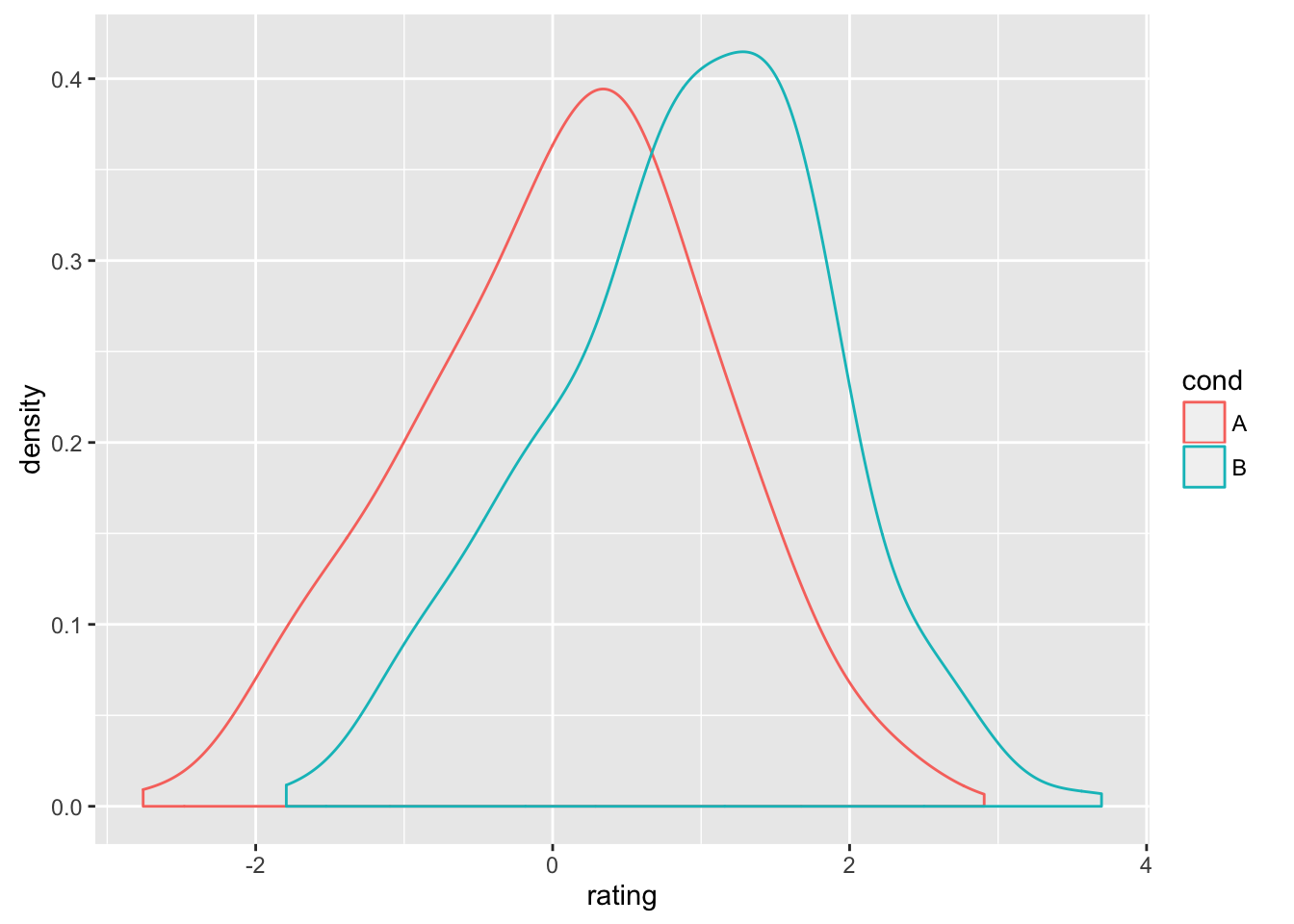
set.seed(1492)
dat <- data.frame(cond = factor(rep(c("A","B"), each=200)),
                   rating = c(rnorm(200),rnorm(200, mean=.8)))

ggplot(dat, aes(x=rating, color=cond)) + geom_bkde(alpha=0)
#> Bandwidth not specified. Using '0.36', via KernSmooth::dpik.
#> Bandwidth not specified. Using '0.31', via KernSmooth::dpik.
ggplot(dat, aes(x=rating, fill=cond)) + geom_bkde(alpha=0.3)
#> Bandwidth not specified. Using '0.36', via KernSmooth::dpik.
#> Bandwidth not specified. Using '0.31', via KernSmooth::dpik.

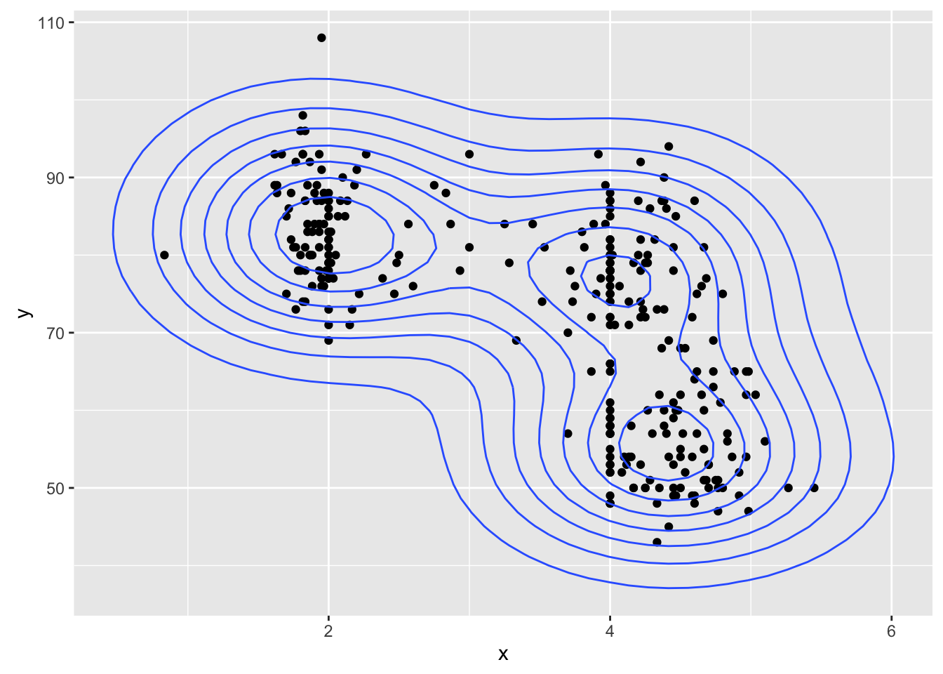
# 2D KernSmooth::bkde2D plots are a WIP

geyser_dat <- data.frame(x=geyser$duration, y=geyser$waiting)

ggplot(geyser_dat, aes(x, y)) +
  geom_point() +
  geom_bkde2d(bandwidth=c(0.7, 7))
ggplot(geyser_dat, aes(x, y)) +
  geom_point() +
  stat_bkde2d(bandwidth=c(0.7, 7))

# coord_proj LIVES! (still needs work)

world <- map_data("world")
world <- world[world$region != "Antarctica",]

gg <- ggplot()
gg <- gg + geom_map(data=world, map=world,
                    aes(x=long, y=lat, map_id=region))
gg <- gg + coord_proj("+proj=wintri")
gg

# stat_ash + compare density plots

set.seed(1492)
dat <- data.frame(x=rnorm(100))
grid.arrange(ggplot(dat, aes(x)) + stat_ash(),
             ggplot(dat, aes(x)) + stat_bkde(),
             ggplot(dat, aes(x)) + stat_density(),
             nrow=3)
#> Estimate nonzero outside interval ab.
#> Bandwidth not specified. Using '0.43', via KernSmooth::dpik.

cols <- RColorBrewer::brewer.pal(3, "Dark2")
ggplot(dat, aes(x)) +
  stat_ash(alpha=1/2, fill=cols[3]) +
  stat_bkde(alpha=1/2, fill=cols[2]) +
  stat_density(alpha=1/2, fill=cols[1]) +
  geom_rug() +
  labs(x=NULL, y="density/estimate") +
  scale_x_continuous(expand=c(0,0)) +
  theme_bw() +
  theme(panel.grid=element_blank()) +
  theme(panel.border=element_blank())
#> Estimate nonzero outside interval ab.
#> Bandwidth not specified. Using '0.43', via KernSmooth::dpik.

Test Results
library(ggalt)
library(testthat)

date()
#> [1] "Sun Sep 13 07:22:24 2015"

test_dir("tests/")
#> testthat results ========================================================================================================
#> OK: 0 SKIPPED: 0 FAILED: 0
#>
#> DONE
Code of Conduct
Please note that this project is released with a Contributor Code of Conduct. By participating in this project you agree to abide by its terms.