You can not select more than 25 topics
Topics must start with a letter or number, can include dashes ('-') and can be up to 35 characters long.
|
|
8 years ago | |
|---|---|---|
| R | 8 years ago | |
| README_figs | 8 years ago | |
| inst/fonts | 8 years ago | |
| man | 8 years ago | |
| tests | 9 years ago | |
| .Rbuildignore | 8 years ago | |
| .gitignore | 8 years ago | |
| .travis.yml | 8 years ago | |
| CONDUCT.md | 9 years ago | |
| DESCRIPTION | 8 years ago | |
| LICENSE | 9 years ago | |
| NAMESPACE | 8 years ago | |
| NEWS | 8 years ago | |
| README.Rmd | 8 years ago | |
| README.html | 8 years ago | |
| README.md | 8 years ago | |
| ggalt.Rproj | 9 years ago | |
README.md


ggalt : Extra Coordinate Systems, Geoms and Statistical Transformations for 'ggplot2'
A compendium of 'geoms', 'coords' and 'stats' for 'ggplot2', including splines, 1d and 2d densities, univariate average shifted histograms and a new map coordinate system based on the 'PROJ.4'-library.
The first three forays into this brave, new ggplot2 world are splines! and being able to use the (much better) KernSmooth::bkde and KernSmooth::bkde2D for density plots and an initial port of the (still needing work) coord_proj.
The following functions are implemented:
coord_proj: Likecoord_maponly better 😜geom_xspline: Connect control points/observations with an X-splinestat_xspline: Connect control points/observations with an X-splinegeom_bkde: Display a smooth density estimate (usesKernSmooth::bkde)stat_bkde: Display a smooth density estimate (usesKernSmooth::bkde)geom_bkde2d: Contours from a 2d density estimate. (usesKernSmooth::bkde2D)stat_bkde2d: Contours from a 2d density estimate. (usesKernSmooth::bkde2D)stat_ash: Compute and display a univariate averaged shifted histogram (polynomial kernel) (usesash::ash1/ash::bin1)scale_color_pokemon:scale_fill_pokemon: discrete pokemon scales (data taken from the hard work by the http://www.pokegraphs.com/)byte_format: + helpers. e.g. turn10000into10 Kb
News
- Version 0.1.5.9000 - Pokemon discrete color scales!
- Version 0.1.2.9000 - Fixed bug with limits not working in coord_proj thx to @mstrimas
- Version 0.1.1 - CRAN!
- Version 0.1.0.9000 - Tweaks for ggplot2 2.0 release
- Version 0.0.4.9000 -
stat_ash - Version 0.0.3.9000 -
coord_proj! (requires my github copy of ggplot2 for now) - Version 0.0.2.9005 - cleanup before blog post
- Version 0.0.2.9002 - working 2D density plots
- Version 0.0.2.9000 initial release
Installation
# you'll want to see the vignettes, trust me
install.packages("ggplot2")
install.packages("ggalt")
# OR: devtools::install_github("hrbrmstr/ggalt")
Usage
library(ggplot2)
library(gridExtra)
library(ggalt)

# current verison
packageVersion("ggalt")
#> [1] '0.2.0.9000'

set.seed(1492)
dat <- data.frame(x=c(1:10, 1:10, 1:10),
                  y=c(sample(15:30, 10), 2*sample(15:30, 10), 3*sample(15:30, 10)),
                  group=factor(c(rep(1, 10), rep(2, 10), rep(3, 10)))
)
Splines!
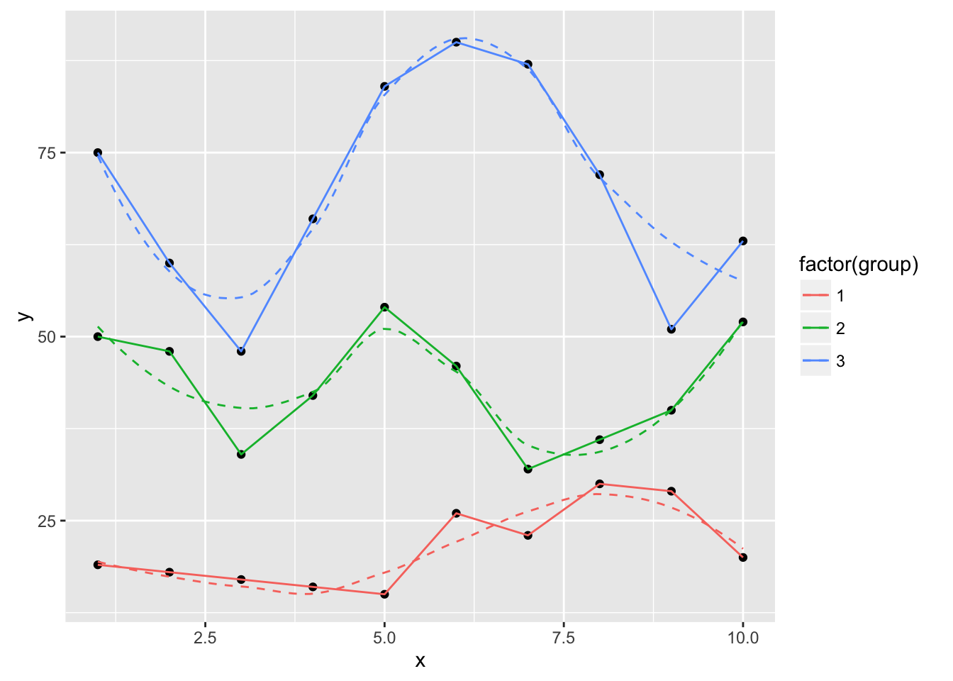
ggplot(dat, aes(x, y, group=group, color=group)) +
  geom_point() +
  geom_line()

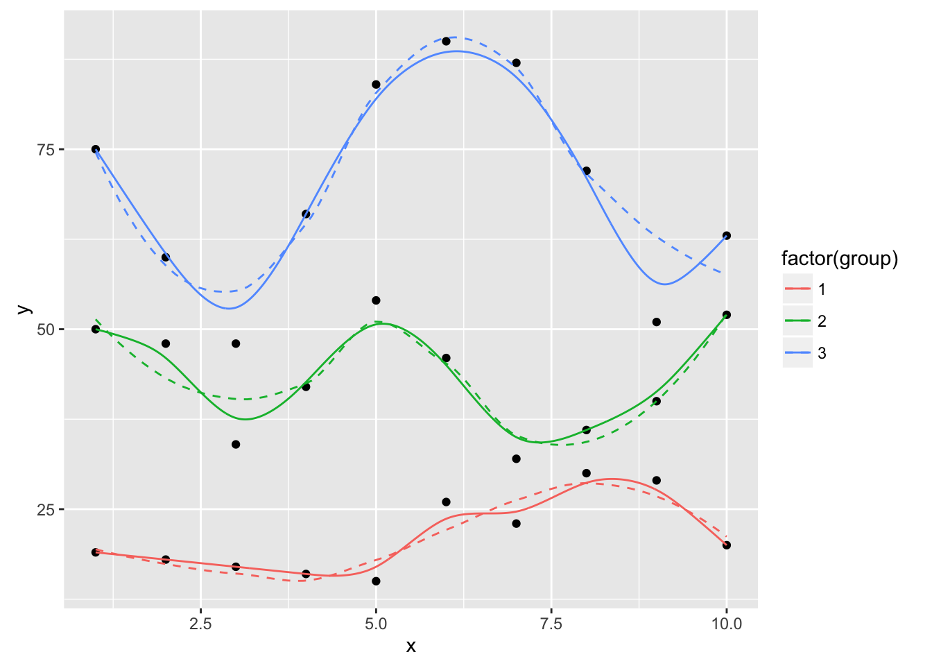
ggplot(dat, aes(x, y, group=group, color=factor(group))) +
  geom_point() +
  geom_line() +
  geom_smooth(se=FALSE, linetype="dashed", size=0.5)

ggplot(dat, aes(x, y, group=group, color=factor(group))) +
  geom_point(color="black") +
  geom_smooth(se=FALSE, linetype="dashed", size=0.5) +
  geom_xspline(size=0.5)

ggplot(dat, aes(x, y, group=group, color=factor(group))) +
  geom_point(color="black") +
  geom_smooth(se=FALSE, linetype="dashed", size=0.5) +
  geom_xspline(spline_shape=-0.4, size=0.5)

ggplot(dat, aes(x, y, group=group, color=factor(group))) +
  geom_point(color="black") +
  geom_smooth(se=FALSE, linetype="dashed", size=0.5) +
  geom_xspline(spline_shape=0.4, size=0.5)

ggplot(dat, aes(x, y, group=group, color=factor(group))) +
  geom_point(color="black") +
  geom_smooth(se=FALSE, linetype="dashed", size=0.5) +
  geom_xspline(spline_shape=1, size=0.5)
ggplot(dat, aes(x, y, group=group, color=factor(group))) +
  geom_point(color="black") +
  geom_smooth(se=FALSE, linetype="dashed", size=0.5) +
  geom_xspline(spline_shape=0, size=0.5)
ggplot(dat, aes(x, y, group=group, color=factor(group))) +
  geom_point(color="black") +
  geom_smooth(se=FALSE, linetype="dashed", size=0.5) +
  geom_xspline(spline_shape=-1, size=0.5)

Alternate (better) density plots
# bkde

data(geyser, package="MASS")

ggplot(geyser, aes(x=duration)) +
  stat_bkde(alpha=1/2)
#> Bandwidth not specified. Using '0.14', via KernSmooth::dpik.

ggplot(geyser, aes(x=duration)) +
  geom_bkde(alpha=1/2)
#> Bandwidth not specified. Using '0.14', via KernSmooth::dpik.

ggplot(geyser, aes(x=duration)) +
  stat_bkde(bandwidth=0.25)

ggplot(geyser, aes(x=duration)) +
  geom_bkde(bandwidth=0.25)

set.seed(1492)
dat <- data.frame(cond = factor(rep(c("A","B"), each=200)),
                   rating = c(rnorm(200),rnorm(200, mean=.8)))

ggplot(dat, aes(x=rating, color=cond)) + geom_bkde(fill="#00000000")
#> Bandwidth not specified. Using '0.36', via KernSmooth::dpik.
#> Bandwidth not specified. Using '0.31', via KernSmooth::dpik.

ggplot(dat, aes(x=rating, fill=cond)) + geom_bkde(alpha=0.3)
#> Bandwidth not specified. Using '0.36', via KernSmooth::dpik.
#> Bandwidth not specified. Using '0.31', via KernSmooth::dpik.

# ash

set.seed(1492)
dat <- data.frame(x=rnorm(100))
grid.arrange(ggplot(dat, aes(x)) + stat_ash(),
             ggplot(dat, aes(x)) + stat_bkde(),
             ggplot(dat, aes(x)) + stat_density(),
             nrow=3)
#> Estimate nonzero outside interval ab.
#> Bandwidth not specified. Using '0.43', via KernSmooth::dpik.

cols <- RColorBrewer::brewer.pal(3, "Dark2")
ggplot(dat, aes(x)) +
  stat_ash(alpha=1/3, fill=cols[3]) +
  stat_bkde(alpha=1/3, fill=cols[2]) +
  stat_density(alpha=1/3, fill=cols[1]) +
  geom_rug() +
  labs(x=NULL, y="density/estimate") +
  scale_x_continuous(expand=c(0,0)) +
  theme_bw() +
  theme(panel.grid=element_blank()) +
  theme(panel.border=element_blank())
#> Estimate nonzero outside interval ab.
#> Bandwidth not specified. Using '0.43', via KernSmooth::dpik.

Alternate 2D density plots
m <- ggplot(faithful, aes(x = eruptions, y = waiting)) +
       geom_point() +
       xlim(0.5, 6) +
       ylim(40, 110)

m + geom_bkde2d(bandwidth=c(0.5, 4))

m + stat_bkde2d(bandwidth=c(0.5, 4), aes(fill = ..level..), geom = "polygon")

coord_proj LIVES! (still needs a teensy bit of work)
world <- map_data("world")
#>
#>  # ATTENTION: maps v3.0 has an updated 'world' map.        #
#>  # Many country borders and names have changed since 1990. #
#>  # Type '?world' or 'news(package="maps")'. See README_v3. #
world <- world[world$region != "Antarctica",]

gg <- ggplot()
gg <- gg + geom_map(data=world, map=world,
                    aes(x=long, y=lat, map_id=region))
gg <- gg + coord_proj("+proj=wintri")
gg

ProPublica StateFace
# Run show_stateface() to see the location of the TTF StateFace font
# You need to install it for it to work

set.seed(1492)
dat <- data.frame(state=state.abb,
                  x=sample(100, 50),
                  y=sample(100, 50),
                  col=sample(c("#b2182b", "#2166ac"), 50, replace=TRUE),
                  sz=sample(6:15, 50, replace=TRUE),
                  stringsAsFactors=FALSE)
gg <- ggplot(dat, aes(x=x, y=y))
gg <- gg + geom_stateface(aes(label=state, color=col, size=sz))
gg <- gg + scale_color_identity()
gg <- gg + scale_size_identity()
gg

Encircling points automagically
d <- data.frame(x=c(1,1,2),y=c(1,2,2)*100)

gg <- ggplot(d,aes(x,y))
gg <- gg + scale_x_continuous(expand=c(0.5,1))
gg <- gg + scale_y_continuous(expand=c(0.5,1))

gg + geom_encircle(s_shape=1, expand=0) + geom_point()

gg + geom_encircle(s_shape=1, expand=0.1, colour="red") + geom_point()

gg + geom_encircle(s_shape=0.5, expand=0.1, colour="purple") + geom_point()

gg + geom_encircle(data=subset(d, x==1), colour="blue", spread=0.02) +
  geom_point()

gg +geom_encircle(data=subset(d, x==2), colour="cyan", spread=0.04) +
  geom_point()

gg <- ggplot(mpg, aes(displ, hwy))
gg + geom_encircle(data=subset(mpg, hwy>40)) + geom_point()

ss <- subset(mpg,hwy>31 & displ<2)

gg + geom_encircle(data=ss, colour="blue", s_shape=0.9, expand=0.07) +
  geom_point() + geom_point(data=ss, colour="blue")

Code of Conduct
Please note that this project is released with a Contributor Code of Conduct. By participating in this project you agree to abide by its terms.